New York City Data Analyzing
drug_overdose = read_csv("./data/VSRR_Provisional_Drug_Overdose_Death_Counts.csv") %>%
  janitor::clean_names()

state_level = c(state.name[1:8], "District of Columbia", state.name[9:32],"New York City", state.name[33:50])

drug_overdose_52 =
  drug_overdose %>%
  filter(!(state_name %in% c("United States"))) %>%
  relocate(state_name) %>%
  mutate(month = factor(month, levels = month.name),
         year = factor(year),
         state_name = factor(state_name, levels = state_level)) %>%
  arrange(state_name) %>%
  group_by(state_name, year) %>%
  mutate(month = sort(month))

nyc_df =
  drug_overdose_52 %>%
  filter(state_name == "New York City")

drug_percent_specified =
  nyc_df %>%
  ungroup() %>%
  select(year, month, indicator, data_value) %>%
  filter(indicator == "Percent with drugs specified")
By Drug Type
Number of Drug Overdose Deaths by Drug Categories in NYC
For nyc_drug_overdose_death dataset: The dimension of this dataset is (912, 12). The percentages with drugs specified for each month from 2015-2021 in NYC are all above 98%, hence, the drugs’ specified data are accurate enough and can be used further. However, the data of death counts for specific drug types in the years 2016 and 2017 are missing.
summarize_nyc_drug =
  nyc_df %>%
  ungroup() %>%
  select(year, month, indicator, data_value) %>%
  filter(!(indicator %in% c("Number of Deaths","Number of Drug Overdose Deaths","Percent with drugs specified"))) %>%
  filter(!(year %in% c("2016","2017"))) %>%
  mutate(indicator = as.factor(indicator)) %>%
  mutate(
    indicator = fct_reorder(indicator, data_value)
  )

summarize_nyc_drug %>%
  ggplot(aes(x = indicator, y = data_value, fill = indicator)) +
  geom_violin(alpha = 0.5) +
  scale_x_discrete(labels = c("Psychostimulants \n with abuse potential \n (T43.6)", "Methadone \n (T40.3)", "Natural & \n semi-synthetic  \n opioids \n (T40.2)", "Natural & semi-\n synthetic opioids, \n incl. methadone \n (T40.2, T40.3)", "Heroin \n (T40.1)", "Cocaine \n (T40.5)", "Synthetic opioids, \n excl. \n methadone \n (T40.4)", "Natural, \n semi-synthetic, & \n synthetic opioids, \n incl. methadone \n (T40.2-T40.4)", "Opioids \n (T40.0-T40.4,\n T40.6)")) +
  guides(fill = guide_legend(nrow = 6, byrow = TRUE)) +
  labs(
    title = "Number of Drug Overdose Deaths by Drug Categories in NYC (2015 - 2021)",
    x = "Drug Categories",
    y = "Number of Drug Overdose Deaths",
    caption = "Data comes from VSRR_Provisional_Drug_Overdose_Death_Counts dataset."
  )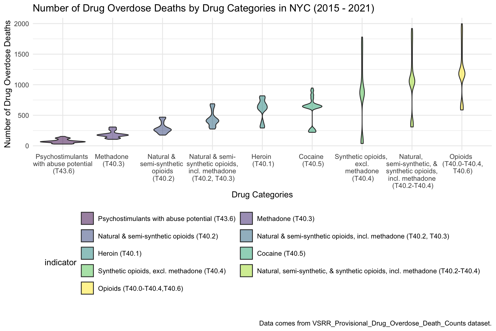
Based on the above Number of Drug Overdose Deaths by Drug Categories plot, in New York City, from 2015 to 2021, the number of people who have died because of overdoses of opioids(T40.0-T40.4, T40.6) has reached nearly 2,000, which indicates that the cause of the highest number of drug overdose deaths is synthetic opioids. Based on the overall shape and distribution of all drug categories, there are more outliers in opioids(T40.0-T40.4, T40.6), synthetic opioids, excl. methadone(T40.4), and Natural, semi-synthetic, & synthetic opioids, incl. methadone(T40.2-T40.4).
By Year
Percent of Drug Overdose Deaths over Total Number of Deaths by Year in NYC
nyc_drug_overdose_death_df =
  nyc_df %>%
  ungroup() %>%
  select(year, month, indicator, data_value) %>%
  filter(indicator %in% c("Number of Deaths", "Number of Drug Overdose Deaths")) %>%
  pivot_wider(
    names_from = indicator,
    values_from = data_value
  ) %>%
  janitor::clean_names() %>%
  group_by(year, month) %>%
  mutate(
    percent_overdose_death = number_of_drug_overdose_deaths / number_of_deaths
  )

nyc_drug_overdose_death_df %>%
  ungroup() %>%
  ggplot(aes(x = month, y = percent_overdose_death, color = year)) +
  geom_point() +
  geom_line(aes(group = year)) +
  labs(
    title = "Percent of Drug Overdose Deaths over Total Number of Deaths by Year in NYC",
    x = "Months",
    y = "Percent of Drug Overdose Deaths",
    caption = "Data comes from VSRR_Provisional_Drug_Overdose_Death_Counts dataset from 2015 to 2021)."
  )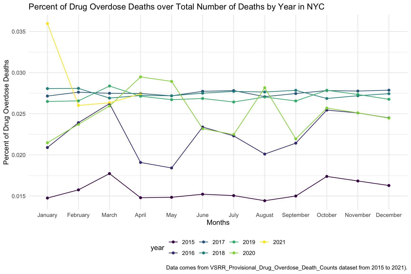
Based on the above Percent of Drug Overdose Deaths over Total Number of Deaths by Year plot, in New York City, the year 2015 has the lowest percentage of drug overdose death with a steady performance. In the years 2016 and 2020, both plots have huge oscillations. The percentages of drug overdose death intensely drop in March and Jun in 2016, and May and August in 2020, and rising again in May and August in 2016, and July and September in 2020. And in the years 2017, 2018, and 2019, the percentages are steady across the year. There may be a time lag in data obtained in 2021, hence the data in this year are not reliable.
nyc_drug_overdose_death_df %>%
  ungroup() %>%
  ggplot(aes(x = month, y = percent_overdose_death, group = NA, color = year)) +
  geom_point() +
  geom_line() +
  facet_grid(.~ year) +
  labs(
    title = "Percent of Drug Overdose Deaths over Total Number of Deaths by Year in NYC",
    x = "Months",
    y = "Percent of Drug Overdose Deaths",
    caption = "Data comes from VSRR_Provisional_Drug_Overdose_Death_Counts dataset from 2015 to 2021."
  ) +
theme(axis.text.x = element_text(angle = 90, hjust = 1)) 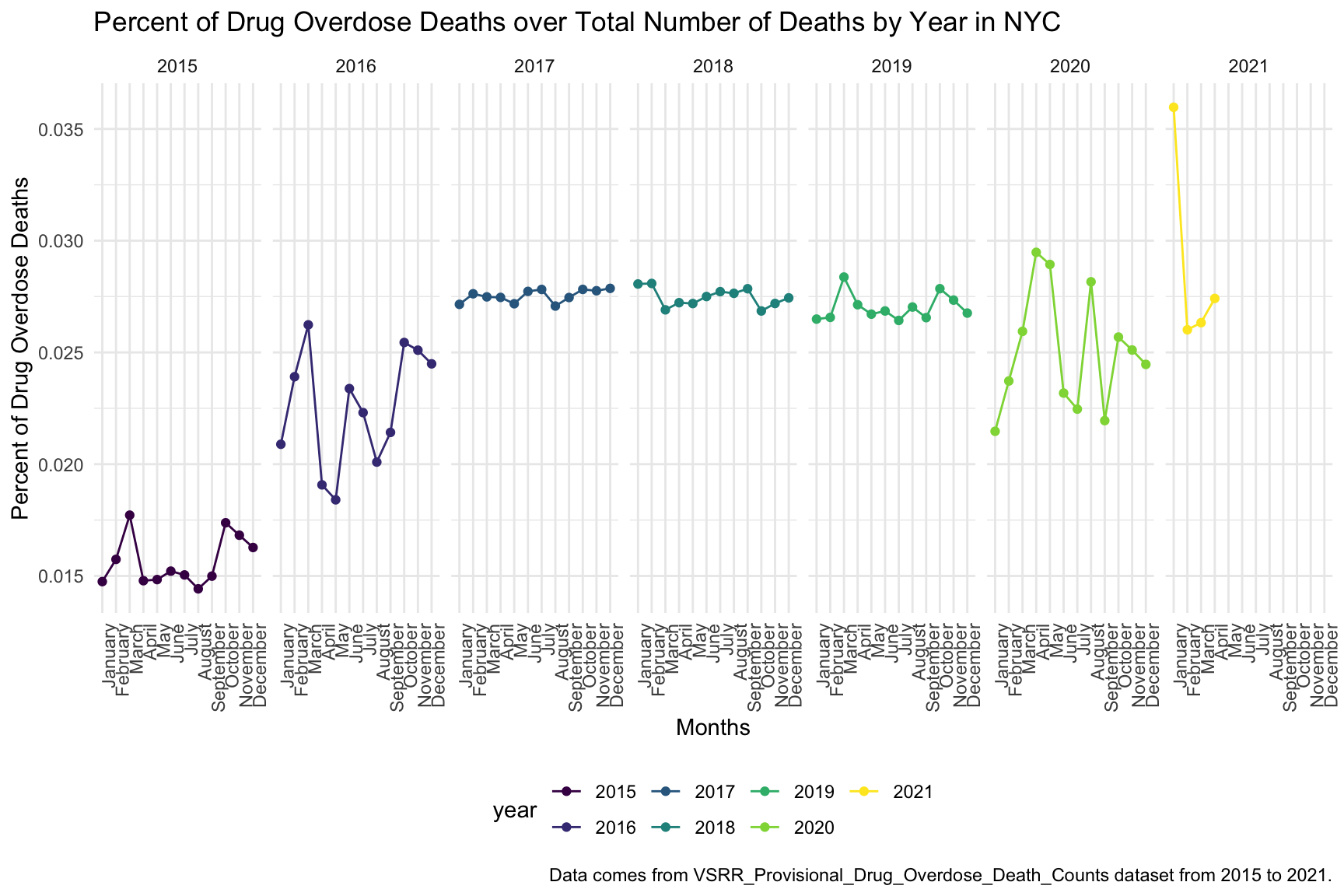
In order to see the trending of percent of drug overdose deaths in the past seven years from 2015 to 2021, we lined up all graphs over the years for comparison. Based on the above scatter plot, we can see that overall the percent of drug overdose deaths shows a tendency to increase by each year. Since there may be a time lag in data obtained in 2021, we ignored the data this year. And the value of the percent of drug overdose deaths has increased from around 0.015 in the year 2015 to around 0.027 in the year 2020.
Drug ~ Year
Number of Drug Overdose Deaths with Drug Categories by Year in NYC
summarize_nyc_drug %>%
  ggplot(aes(x = year, y = data_value, color = indicator)) +
  geom_point() +
  geom_line(aes(group = indicator)) +
  scale_color_viridis(discrete = TRUE, labels = c("Psychostimulants with abuse potential (T43.6)", "Methadone (T40.3)", "Natural & semi-synthetic opioids (T40.2)", "Natural & semi-synthetic opioids, incl. methadone (T40.2, T40.3)", "Heroin (T40.1)", "Cocaine (T40.5)", "Synthetic opioids, excl. methadone (T40.4)", "Natural, semi-synthetic, & synthetic opioids, incl. methadone (T40.2-T40.4)", "Opioids (T40.0-T40.4,T40.6)")) +
  guides(color = guide_legend(nrow = 6, byrow = TRUE)) +
  labs(
    title = "Number of Drug Overdose Deaths with Drug Categories by Year in NYC",
    x = "Drug Categories",
    y = "Number of Drug Overdose Deaths",
    caption = "Data comes from VSRR_Provisional_Drug_Overdose_Death_Counts dataset between 2015 and 2021."
  )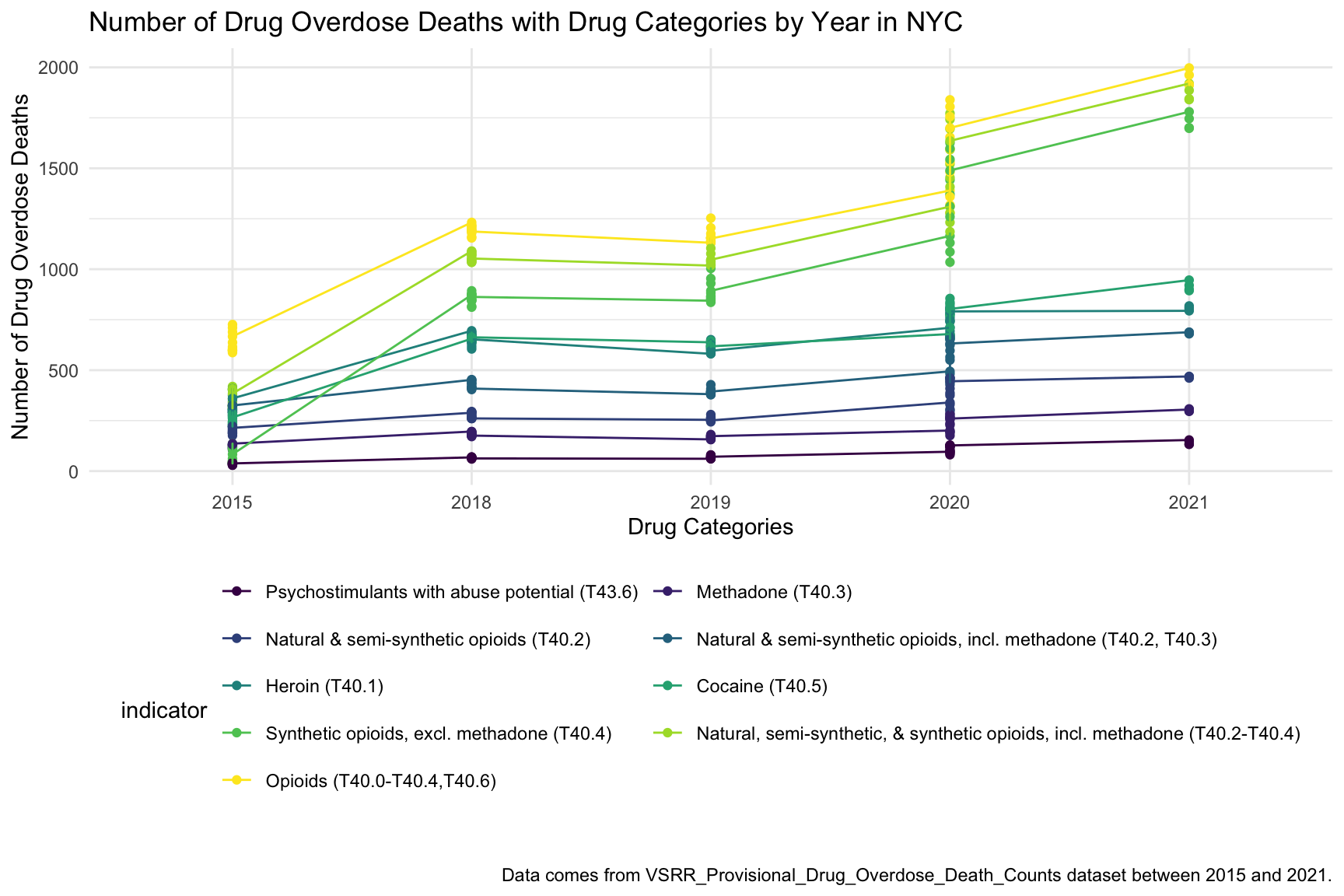
After comparing drug overdose deaths by drug categories and drug overdose deaths by years from 2015 to 2021, now we want to compare the number of drug overdose death both by drug types and by year in New York City. Based on the above scatter plot we can see that the number of death is steadily rising each year for each type of drug. Opioids(T40.0-T40.4, T40.6) has made the highest number of people’s death in 9 types of drug categories since 2015, which indicates that synthetic opioids are the primary cause of people’s death in the case of a drug overdose.
By Age-group & Race
age-adjusted drug overdose death rate by race
ny_drugoverdose_death_by_age =
  read_csv("./data/ny_agegroup_race_state_year_99-19.csv") %>%
  janitor::clean_names() %>%
  #filter(year == (2015:2019)) %>%
  mutate(county = str_replace(county, " County, NY", ""),
         ten_year_age_groups = gsub("years", "", ten_year_age_groups)) %>%
  select(county, year, ten_year_age_groups, race, deaths, population) %>%
  filter(str_detect(county, "Bronx|Queens|Kings|New York|Richmond")) %>%
  mutate(year = factor(year),
         crude_rate = deaths/population * 100000) %>%
  group_by(race)
Next, we want to compare the age-adjusted drug overdose death rate by race in NYC. In order to examine the relationship between drug overdose death, age-group, and race in NYC. We obtained this ny_agegroup_race_state_year_99-19.csv dataset from CDC wonder and calculated the age-adjusted mortality rate by dividing the number of deaths by the population and multiplying by 100000. The dimension of this dataset is (609, 7).
ny_drugoverdose_death_by_age %>%
  ggplot(aes(x = ten_year_age_groups, y = crude_rate, fill = county)) +
  geom_boxplot(outlier.shape = NA, alpha = 0.5) +
  facet_grid(~race) +
  labs(
    title = "Age-Adjusted Drug Overdose Mortality Rate by Race in NYC",
    x = "Age Groups",
    y = "Age-Adjusted Mortality Rate \n(per 100,000)",
    caption = "Source: NYC drug overdose death counts from CDC, 2015-2019"
  )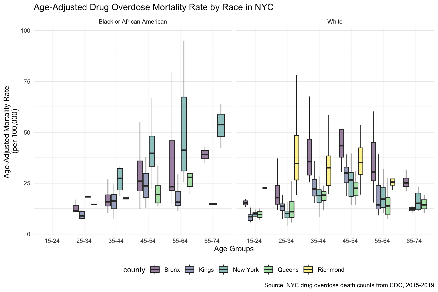
Based on the above age-adjusted drug overdose death rate by race plot, we can see that for black or African Americans, people among age 55-64 have the highest death rate; and for white, people among age 25-34 have the highest death rate. Black or African Americans have the highest death rate in New York county, and white people have the highest death rate in Richmond county.
By Income
Median Household Income: New York vs. The U.S
ny_eco_df =
  read_csv("./data/median_household_income_ny.csv") %>%
  janitor::clean_names() %>%
  select(year, household_income_by_race, household_income_by_race_moe, geography) %>%
  filter(year >= "2015",
         !(geography  %in% c("New York-Newark-Jersey City, NY-NJ-PA", "New York"))) %>%
  mutate(
    geography = str_replace(geography, "New York, NY", "New York City"),
    geography = str_replace(geography, ", NY", ""),
    year = factor(year))
For nyc_median_household_income dataset: In order to examine the relationship between drug overdose death and income in NYC. We obtained this median_household_income_ny.csv dataset from DATA USA, chose years after 2015, and selected all five counties in New York City. The dimension of this dataset is (35, 4).
ny_eco_df %>%
  mutate(text_label = str_c("Year: ", year, "\nMedian Household Income: $", household_income_by_race,
                            "\nMargin of error: ± $", household_income_by_race_moe)) %>%
  plot_ly(
    x = ~year, y = ~household_income_by_race, color = ~geography, text = ~text_label,
    alpha = 0.5, type = "scatter", mode = "markers+lines", colors = "viridis",error_y = ~list(array = household_income_by_race_moe)) %>%
  layout(
    title = "Median Household Income: New York vs. The U.S",
         xaxis = list(title = "Year"),
         yaxis = list(title = "Median Household Income"))
From the above plotly, we can see that all the median household incomes in New York counties are higher than the median household income in the overall United States. And New York county has the highest median household income in all five counties in NYC.
Income vs. Percent of Drug Overdose Death by Year in NYC
income_drug_df_ny =
  nyc_drug_overdose_death_df %>%
    ungroup() %>%
    group_by(year) %>%
    summarize(overdose_death_rate = sum(number_of_drug_overdose_deaths)/sum(number_of_deaths)) %>%
    inner_join(., ny_eco_df %>% filter(geography %in% "New York City"))

year_death =
  income_drug_df_ny %>%
  ggplot(aes(x = year, y = overdose_death_rate, group = NA)) +
  geom_point() +
  geom_line() +
  ggtitle('Drug Overdose Death Rate by Year') +
  labs(
    x = "Year",
    y = "Overdose Death Rate"
  )

income_year =
  income_drug_df_ny %>%
  ggplot(aes(x = year, y = household_income_by_race, group = NA)) +
  geom_point() +
  geom_line() +
  ggtitle('Income by Year') +
  labs(
    x = "Year",
    y = "Household Income"
  )

smooth =
  income_drug_df_ny %>%
  ggplot(aes(x = household_income_by_race, y = overdose_death_rate, group = NA)) +
  geom_point() +
  geom_smooth(method = "lm", se = FALSE, color = "royalblue4") +
  ggtitle('Drug Overdose Death Rate vs. Income') +
   labs(
    x = "Household Income",
    y = "Overdose Death Rate"
  )

(year_death + income_year)/smooth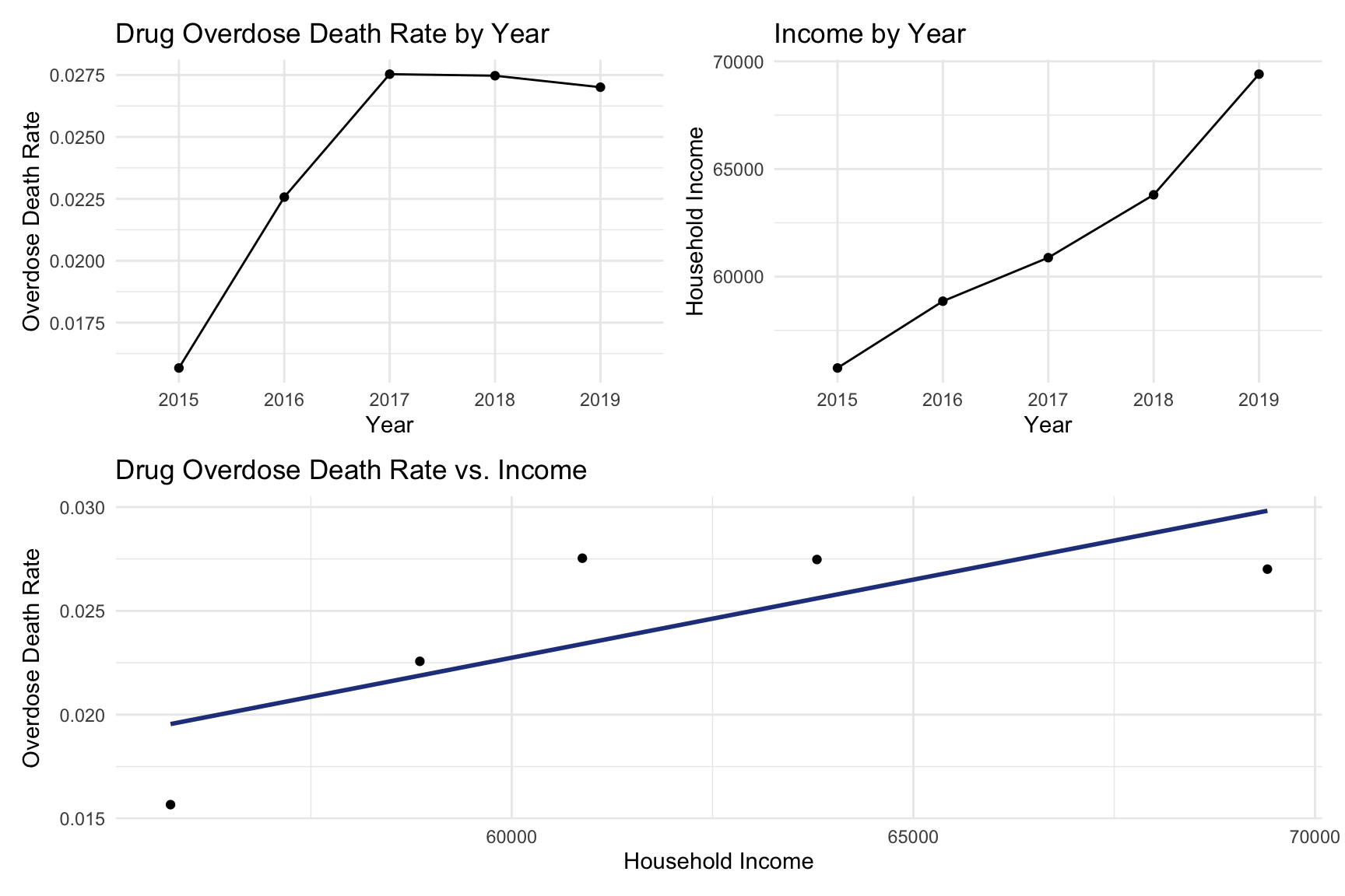
Based on the above income vs. percent of drug overdose death by year, we can see that in NYC, the overdose death rate and household income are positively related. People with a higher income would have a higher drug overdose death rate.
Counties change
ny_county_df =
  read_csv("./data/NCHS_-_Drug_Poisoning_Mortality_by_County__United_States.csv") %>%
  janitor::clean_names() %>%
  filter(state %in% "New York") %>%
  select(year, county, population, model_based_death_rate) %>%
  rename(death_rate = model_based_death_rate) %>%
  mutate(
    county = str_replace(county, "County, NY", "")) %>%
  mutate(year = factor(year),
         county = str_to_lower(county)) %>%
  filter(str_detect(county, "bronx|queens|kings|new york|richmond")) %>%
  mutate(county = str_replace(county, " $", "")) %>%
  relocate(county)


data(county.fips)
nyc_fip = county.fips %>%
  filter(str_detect(polyname, "new york")) %>%
  mutate(
    polyname = str_replace(polyname, "new york,", "")) %>%
  filter(str_detect(polyname, "bronx|queens|kings|new york|richmond")) %>%
  rename(county = polyname) %>%
  as.tibble()

ny_county_df = left_join(ny_county_df,nyc_fip, by = "county")


highlight_county = function(county_fips)
{
  data(county.map, package="choroplethrMaps", envir=environment())
  df = county.map[county.map$region %in% county_fips, ]
  geom_polygon(data=df, aes(long, lat, group = group), color = "yellow", fill = NA, size = 1)
}
add_text_county = function(county_fips){
  data(county.map, package="choroplethrMaps", envir=environment())
  df = county.map[county.map$region %in% county_fips, ]
  #geom_text(data=df, aes(mean(long), mean(lat), label = paste0(str_to_title(pull(county_fips, county)), " County\n", pull(county_fips, death_rate))), color = "white")
  geom_label(data=df, aes(mean(long), mean(lat), label = paste0(str_to_title(pull(county_fips, county)), " County\nDR: ", round(pull(county_fips, death_rate),2))), fill = "white", size = 3)
}
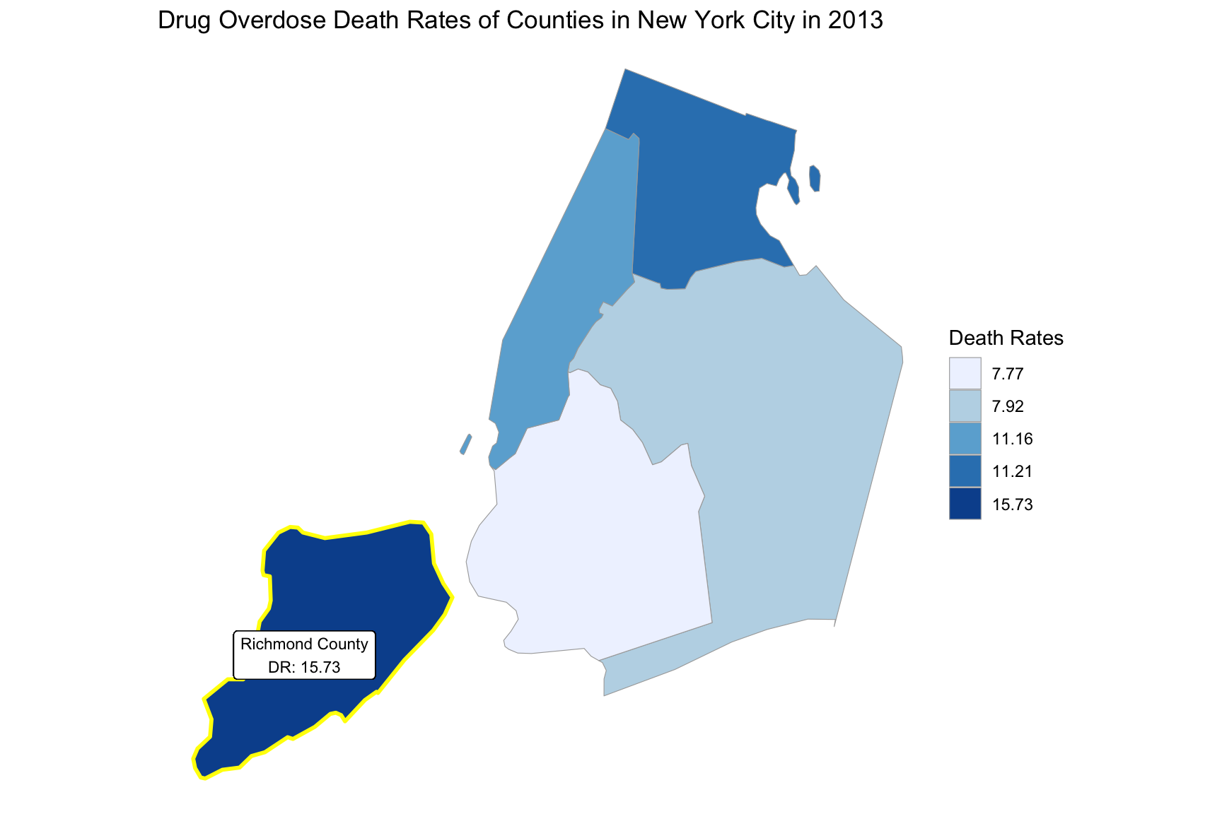
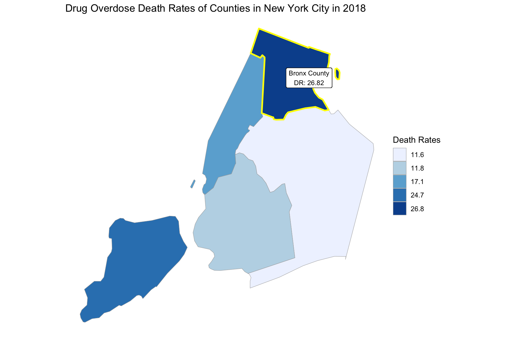
Based on the changes of drug overdose death rates over counties by an interval of 5 years, we can see that in the year 2003, the highest drug overdose death rates occurred in New York county. In the years 2008 and 2013, the highest drug overdose death rates occurred in Richmond county. And in the year 2018, the highest drug overdose death rates occurred in Bronx county.
Counties change, 5-yr interval
2003
year_select = 2003
start_county_df = ny_county_df %>%
  select(county, year, death_rate, fips) %>%
  filter(year == year_select)

start_deathrate_df =
  start_county_df %>%
  rename(region = fips,
        value = death_rate) %>%
  select(value, region)

county_choropleth(start_deathrate_df, title = "Drug Overdose Death Rates of Counties in New York City in 2003",
                    legend = "Death Rates",
                    county_zoom = start_deathrate_df$region) +
highlight_county(start_county_df[which.max(pull(start_county_df, death_rate)),]) +
add_text_county(start_county_df[which.max(pull(start_county_df, death_rate)),])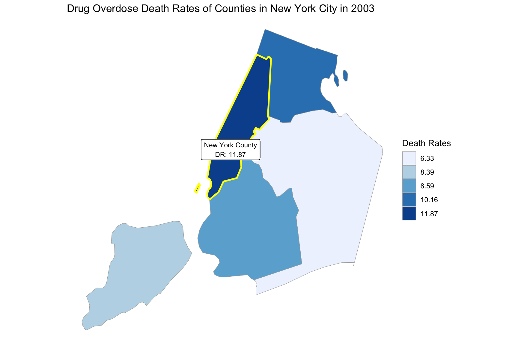
2008
year_select = 2008
start_county_df = ny_county_df %>%
  select(county, year, death_rate, fips) %>%
  filter(year == year_select)

start_deathrate_df =
  start_county_df %>%
  rename(region = fips,
        value = death_rate) %>%
  select(value, region)

county_choropleth(start_deathrate_df, title = "Drug Overdose Death Rates of Counties in New York City in 2008",
                    legend = "Death Rates",
                    county_zoom = start_deathrate_df$region) +
highlight_county(start_county_df[which.max(pull(start_county_df, death_rate)),]) +
add_text_county(start_county_df[which.max(pull(start_county_df, death_rate)),])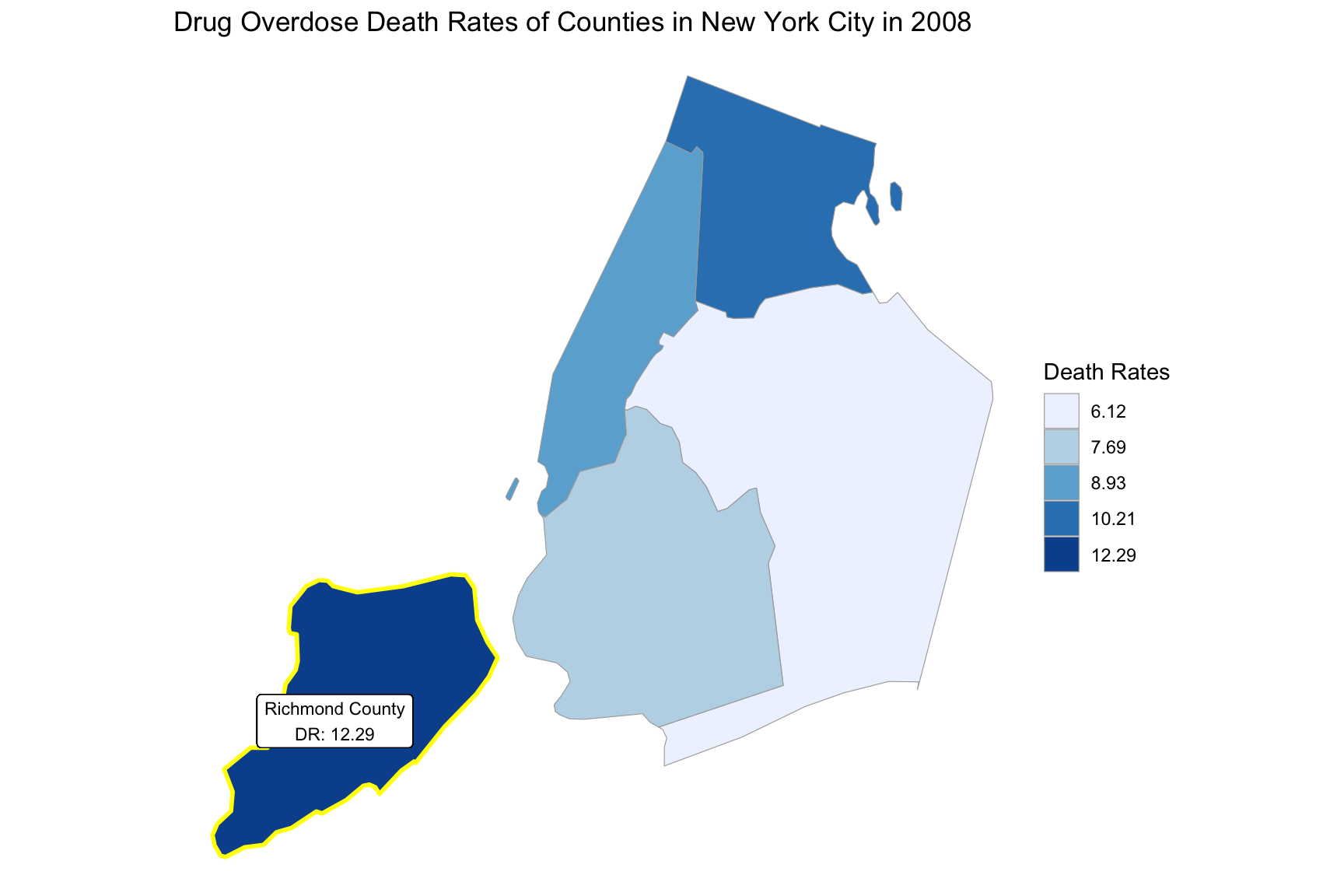
2013
year_select = 2013
start_county_df = ny_county_df %>%
  select(county, year, death_rate, fips) %>%
  filter(year == year_select)

start_deathrate_df =
  start_county_df %>%
  rename(region = fips,
        value = death_rate) %>%
  select(value, region)

county_choropleth(start_deathrate_df, title = "Drug Overdose Death Rates of Counties in New York City in 2013",
                    legend = "Death Rates",
                    county_zoom = start_deathrate_df$region) +
highlight_county(start_county_df[which.max(pull(start_county_df, death_rate)),]) +
add_text_county(start_county_df[which.max(pull(start_county_df, death_rate)),])